Plots Manipulation Guide (Labels, Titles, Colors)

This page demonstrates how to customize labels, titles, subtitles, and colors for each plot type. All images on this page are generated by running examples/plots_manipulation_examples.py.

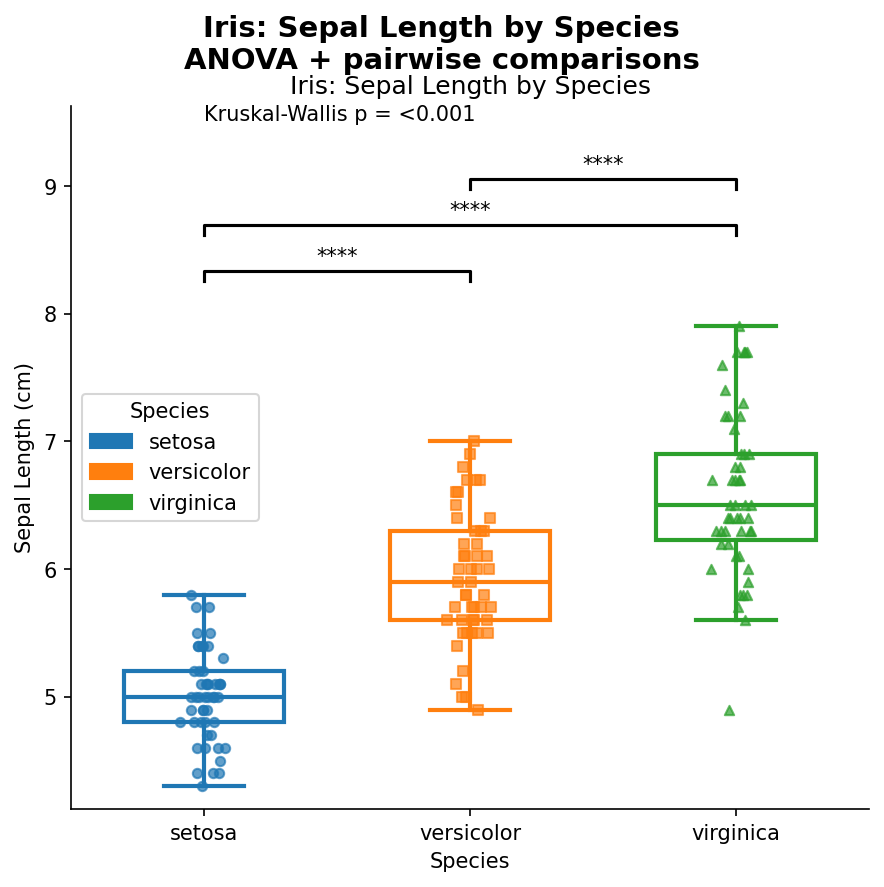
Boxplot

from ggpubpy import plot_boxplot_with_stats, load_iris
import matplotlib.pyplot as plt

iris = load_iris()
fig, ax = plot_boxplot_with_stats(
    df=iris,
    x="species",
    y="sepal_length",
    x_label="Species",
    y_label="Sepal Length (cm)",
    title="Iris: Sepal Length by Species",
    subtitle="ANOVA + pairwise comparisons",
    palette={"setosa": "#1f77b4", "versicolor": "#ff7f0e", "virginica": "#2ca02c"},
)
# Post adjustments (optional)
ax.set_xlabel("Species")
ax.set_ylabel("Sepal Length (cm)")
ax.set_title("Iris: Sepal Length by Species")
fig.savefig("examples/plots_manip_boxplot.png", dpi=150, bbox_inches="tight")

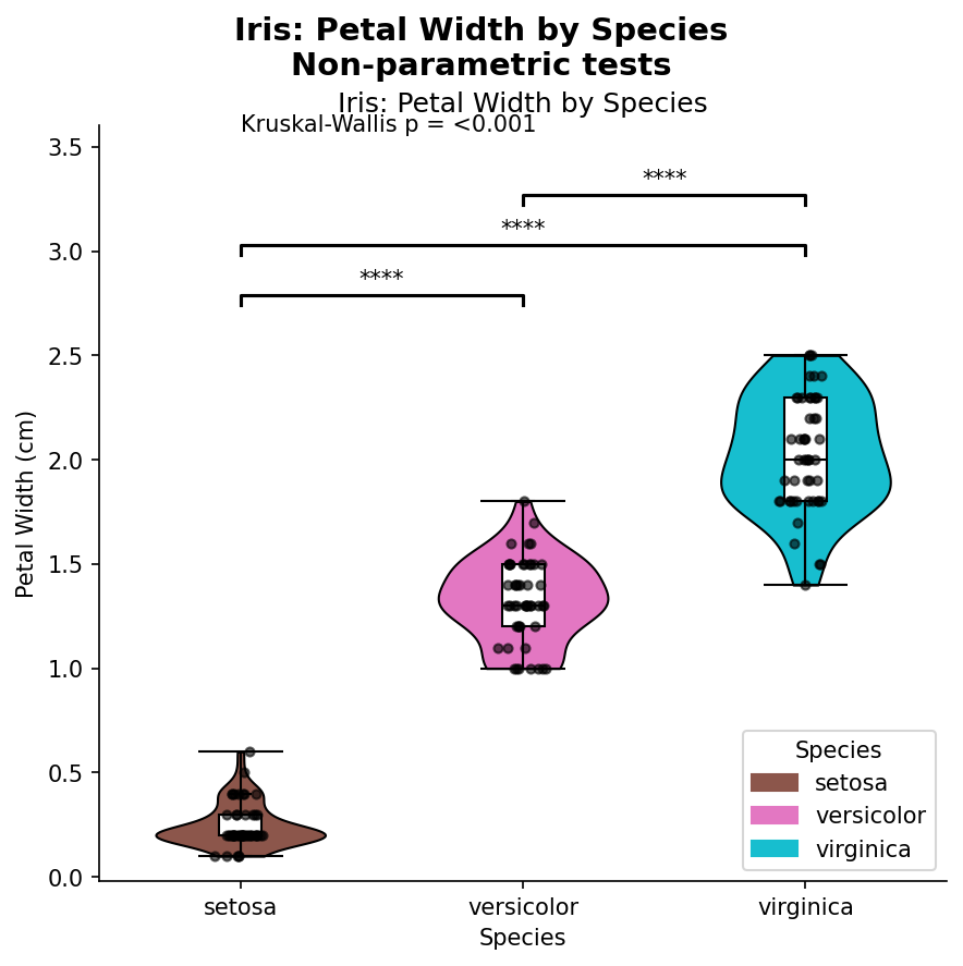
Violin Plot

from ggpubpy import plot_violin_with_stats, load_iris
import matplotlib.pyplot as plt

iris = load_iris()
fig, ax = plot_violin_with_stats(
    df=iris,
    x="species",
    y="petal_width",
    x_label="Species",
    y_label="Petal Width (cm)",
    title="Iris: Petal Width by Species",
    subtitle="Non-parametric tests",
    palette={"setosa": "#8c564b", "versicolor": "#e377c2", "virginica": "#17becf"},
)
ax.set_xlabel("Species")
ax.set_ylabel("Petal Width (cm)")
ax.set_title("Iris: Petal Width by Species")
fig.savefig("examples/plots_manip_violin.png", dpi=150, bbox_inches="tight")

Shift Plot (two-panel control)

from ggpubpy import plot_shift, load_iris
import matplotlib.pyplot as plt

iris = load_iris()
x = iris[iris["species"] == "setosa"]["sepal_length"].values
y = iris[iris["species"] == "versicolor"]["sepal_length"].values

fig = plot_shift(
    x,
    y,
    paired=False,
    show_quantiles=True,
    show_quantile_diff=True,
    x_label="Setosa",
    y_label="Versicolor",
    title="Iris: Setosa vs Versicolor Shift Plot",
    subtitle="Main + quantile differences",
    color="#27AE60",
    line_color="#2C3E50",
)

ax_main, ax_shift = fig.axes
ax_main.set_xlabel("Setosa")
ax_main.set_ylabel("Versicolor")
ax_main.set_title("Iris: Setosa vs Versicolor Shift Plot")
ax_shift.set_xlabel("Setosa quantiles")
ax_shift.set_ylabel("Versicolor - Setosa quantile differences")
fig.savefig("examples/plots_manip_shift.png", dpi=150, bbox_inches="tight")

Correlation Matrix

from ggpubpy import plot_correlation_matrix, load_iris
import matplotlib.pyplot as plt

iris = load_iris()
fig, axes = plot_correlation_matrix(
    df=iris,
    columns=["sepal_length", "sepal_width", "petal_length", "petal_width"],
    title="Iris Dataset - Correlation Matrix",
    subtitle="Pearson correlation with significance",
    color="#2E86AB",
    alpha=0.6,
)
axes[0, 0].set_xlabel("Sepal Length (cm)")
axes[0, 0].set_ylabel("Sepal Length (cm)")
fig.savefig("examples/plots_manip_corr.png", dpi=150, bbox_inches="tight")

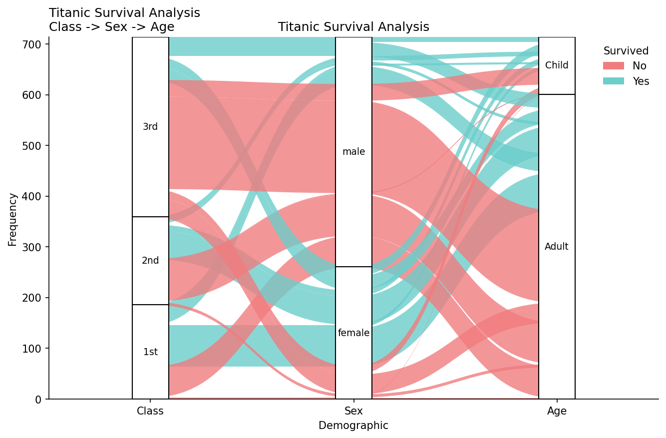
Alluvial Plot

from ggpubpy import plot_alluvial, load_titanic
import pandas as pd
import numpy as np
import matplotlib.pyplot as plt

# Prepare Titanic
titanic = load_titanic()
titanic = titanic.dropna(subset=["Age"])
titanic["Class"] = titanic["Pclass"].map({1: "1st", 2: "2nd", 3: "3rd"})
titanic["AgeCat"] = np.where(titanic["Age"] < 18, "Child", "Adult")
titanic["Survived"] = titanic["Survived"].astype(str).replace({"0": "No", "1": "Yes"})

# Frequency table with IDs
tab = (
    titanic.groupby(["Class", "Sex", "AgeCat", "Survived"]).size().reset_index(name="Freq")
)
tab = tab.rename(columns={"AgeCat": "Age"})
tab["alluvium"] = tab.index

fig, ax = plot_alluvial(
    tab,
    dims=["Class", "Sex", "Age"],
    value_col="Freq",
    color_by="Survived",
    id_col="alluvium",
    x_label="Demographic",
    y_label="Frequency",
    title="Titanic Survival Analysis",
    subtitle="Class -> Sex -> Age",
    color_map={"No": "#F17C7E", "Yes": "#6CCECB"},
)
ax.set_xlabel("Demographic")
ax.set_ylabel("Frequency")
ax.set_title("Titanic Survival Analysis")
fig.savefig("examples/plots_manip_alluvial.png", dpi=150, bbox_inches="tight")